SupplyStream: Synthetic Retail Supply Chain Simulator + Analytics
A realistic, Python-driven simulator that creates a production-style retail supply chain dataset for an Indian retail (apparel, footwear, and accessories) network built on a hub-and-spoke topology with cross-docking, designed to feed directly into a professional Power BI dashboard for analysis across orders, deliveries, costs, inventory, suppliers, and returns
Live interactive demo of the Power BI dashboard
🧭 Executive summary
- Problem: As data enthusiasts, we often need access to realistic supply chain data to explore ideas, build dashboards, and train machine learning models. However, getting sensitive production data can raise privacy concerns and compliance issues, creating barriers to experimentation and slowing down the pace of innovation.
- Approach: Drawing on my industrial experience, I designed a simulated hub-and-spoke supply chain network with a two-tier transport model—specifically tailored for data enthusiasts. This simulation enabled the generation of clean, well-structured fact and dimension tables in CSV format, making them ideal for analytical exploration and machine learning experimentation. These datasets were then integrated into a Power BI model, allowing for rapid prototyping, visualization, and storytelling. This setup also facilitated thorough validation of data integrity and quality, ensuring the synthetic data is both reliable and realistic for practical use.
- Outcome: The result is a rich, synthetic dataset and a reference Power BI dashboard, purpose-built for data enthusiasts. This solution empowers users to test hypotheses, iterate on visualizations, and develop machine learning models in a secure, flexible, and compliant environment. Beyond technical experimentation, it also provides a valuable tool for understanding supply chain dynamics—enabling deeper insights into network behaviour, transport flows, and performance metrics without the constraints of real-world data access.
From Warehouse to Customer: A Complete Order Journey
-
Lets follow a single order through the entire supply chain to understand how the simulation
models
real-world logistics complexity. This example traces an Order from Store ST045 associated with
Bangalore hub, revealing the coordination required when products come from multiple distribution
hubs
- Stage 1: Inventory Positioning
- Before any customer order exists, the hubs (HUB-DEL, HUB-BOM, HUB-BLR) are stocked
by suppliers:
Tiruppur → HUB-DEL (Dresses)
Kanpur → HUB-BOM (Shoes)
Jaipur → HUB-BLR (Accessories) - Behind the code:The gen_suppliers() function creates supplier profiles with reliability scores between 85-98%, while seed_inventory() initializes hub stock levels based on target inventory and reorder points calculated in gen_products(). Daily replenishment logic in main() triggers inbound shipments whenever inventory falls below the reorder point, simulating realistic procurement cycles
- Before any customer order exists, the hubs (HUB-DEL, HUB-BOM, HUB-BLR) are stocked
by suppliers:
- Stage 2: Order Creation
- Store ST045 places an order requiring three items from different hubs:
1 Silk Anarkali 👗 (Dress → HUB-DEL)
1 Leather Loafers 👞 (Shoes → HUB-BOM)
1 Silver Jhumkas 📿 (Accessory → HUB-BLR)
Since the store's home hub is HUB-BLR, only the accessories are locally available—the
other items (shoes and dresse) must come from different hub before consolidation.
- Behind the code: Daily order generation in the main() loop applies multiplicative demand factors based on quarter (Diwali season +80%), month, weekday, and store type. A flagship store in Mumbai generates 2.5x baseline demand compared to a small town outlet, creating realistic geographic demand patterns.
- Store ST045 places an order requiring three items from different hubs:
- Stage 3: Inventory Allocation
- HUB-DEL has the Dress ✅
HUB-BOM has the Shoes ✅
Store ST045 home hub is HUB-BLR so order will be fulfilled from HUB-BLR, Dress and shoe needs inter-hub shipments.
HUB-BLR → Accessory ✅
If any hub lacks sufficient stock, the system triggers track_backorder() to log unfulfilled demand and queue the order for the next replenishment cycle.
- Behind the code: Inventory checks happen at order line creation, comparing requested quantity against current inv_levels for each product-hub combination. Partial fulfillments are tracked separately from complete backorders, enabling analysis of service level performance by category and time period
- HUB-DEL has the Dress ✅
- Stage 4: Inter-Hub Consolidation
- The dress begins a 2,200 km journey from Delhi to Bangalore, while the shoes travel
985 km from Mumbai.
🚚HUB-DEL → HUB-BLR (Dress)
🚚HUB-BOM → HUB-BLR (Shoes)
The TruckLoadManager class queues both items, waiting until accumulated shipments reach 30% of truck capacity (3,000 kg minimum) before dispatching. Express orders flagged for 3-day delivery bypass this consolidation rule and ship immediately despite lower truck utilization.
Accessory is already at HUB-BLR (home hub), so it does not need inter-hub transfer. - Behind the code: TruckLoadManager.add_shipment_item() queues pending shipments by destination hub, tracking cumulative weight and volume. When process_ready_trucks() executes, it creates shipment legs with transit times calculated from distance ÷ 500 km/day truck speed, and costs based on maximum of actual weight or volumetric weight (volume x 200 kg/m³). Inter-hub transfers incur a 20% cost premium versus final-mile courier rates
- The dress begins a 2,200 km journey from Delhi to Bangalore, while the shoes travel
985 km from Mumbai.
- Stage 5: Cross-Dock Processing
- Both items arrive at HUB-BLR.
Accessory waits at HUB-BLR until other items arrive.
Cross-docking adds 1 day processing before final dispatch. - Behind the code: Order lines are tracked in the pending crossdock dictionary grouped by order ID and destination store. Once all items arrive (len(pending) == total_lines_for_order), the system creates a single final-mile shipment leg consolidating all products. This mimics real warehouse operations where partial orders await completion before customer dispatch.
- Both items arrive at HUB-BLR.
- Stage 6: Final Delivery
- A courier departs HUB-BLR with the complete order, delivering to Store ST045 within 1-2 days based on the 45 km distance. Total elapsed time from order placement to delivery: 7 days. Direct shipments (when products are at the store's home hub) deliver in 1-2 days, while this multi-hub order required longer duration due to consolidation and cross-dock delays
- Behind the code: Final-mile shipments log to fact_shipments.csv with shipment type "final" and courier service details. The link_shipment_orders.csv table connects each shipment leg to specific order lines, enabling drill-down analysis of delivery performance by product category, hub, and urgency flag.
- Stage 7: Returns Processing
- Fourteen days after delivery, the store returns the shoes due to wrong size — a common issue accounting for footwear returns in the dataset. The return travels back to HUB-BLR, undergoes inspection, and re-enters available inventory.
- Behind the code: handle_returns() applies product-category-specific return probabilities (footwear 6%, apparel 5%, accessories 3%) and assigns reasons weighted by category (Wrong Size, Damaged, Changed Mind). Each return logs to fact_returns.csv with return date, reason, processing time, and restocking status. The quantity adds back to inv_levels at the return destination hub, updating available stock for future orders.
- Data Capture
Every step writes to fact tables:
➔ fact_orders.csv → Order lines
➔ fact_shipments.csv → Shipment legs
➔ fact_returns.csv → Returns
➔ fact_inventory_snapshot.csv → Daily inventory
➔ fact_backorders.csv → Unfulfilled demand
🏗️ Architecture in brief
🚚 Logistics Model at a glance
- Network Topology
-
20 specialized suppliers mapped to key manufacturing clusters
- Tiruppur (Cotton Apparel)
- Kanpur (Leather Goods)
- Jaipur (Jewellery)
- 3 regional hubs each specializing in a product category: HUB-DEL (Apparel), HUB-BOM (Footwear), HUB-BLR (Accessories)
- ~100 stores (major/minor) assigned to a “home” hub for fulfillment
- Suppliers mapped to key Indian manufacturing clusters (Tiruppur, Kanpur, Jaipur) by specialty
-
20 specialized suppliers mapped to key manufacturing clusters
- Demand Generation
- ~40 daily orders (Poisson process) over Jan 2022-Jun 2025
- Multi-SKU orders (1-5 lines), 3-10 day delivery window
- Reorder Point (ROP) = lead-time demand + safety stock (95% service level)
- Lead times sampled 3-14 days (μ=7, σ=2)
- Single inbound batch per hub when any SKU falls below ROP
-
Shipment & Transportation Logic
The model simulates two transport tiers:
- Inter-Hub Shipments
- Shipments consolidated and dispatched by truck between hubs. Transit time: calculated by distance (e.g., DEL-BOM: 1400 km, DEL-BLR: 2100 km, BOM-BLR: 1000 km).
- Cost: ₹300 + ₹15/km + ₹8·chargeable_kg, with a 1.2x multiplier for inter-hub bulk shipments.
- Truck capacity: 10,000 kg or 60 m³, minimum load threshold 30%. Express shipments bypass minimum load threshold.
- Final-Mile Shipments
- Direct store shipments: local pick if all lines from same hub or cross-docked consolidation.
- Delivery lead time: 1-2 days for distances ≤100 km, up to 2 days for longer distances.
- Cost uses the same cost function without the inter-hub multiplier.
-
- Returns are simulated with a 3-6% chance per line, random quantity, and category-based reason probabilities.
- Backorders: Unfulfilled order quantities are tracked as backorders, with status and date.
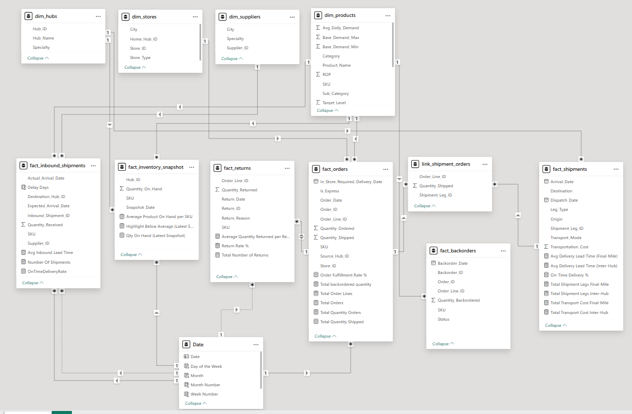
📂 Output of Synthetic Data Generator
- Dimensions:
- dim_hubs.csv
- dim_stores.csv
- dim_products.csv
- dim_suppliers.csv
- Facts:
- fact_orders.csv
- fact_shipments.csv
- fact_inventory_snapshot.csv
- fact_returns.csv
- fact_inbound_shipments.csv
- fact_backorders.csv
- Link: link_shipment_orders.csv
- Logs: SupplyChain_Data/data_gen.log
dim_hubs.csv
Distribution hub master data containing specialization and location details for the three primary fulfillment centers.
| Column Name | Data Type | Description |
|---|---|---|
| Hub_ID PK | String | Unique hub identifier |
| Hub_Name | String | Full descriptive hub name |
| Specialty | String | Product category specialization |
Relationships
- Referenced by fact_orders.Source_Hub_ID
- Referenced by dim_stores.Home_Hub_ID
- Referenced by fact_shipments.Origin / Destination
- Referenced by fact_inventory_snapshot.Hub_ID
- Referenced by fact_inbound_shipments. Destination_Hub_ID
dim_stores.csv
Store master data for 100 retail outlets, including home hub assignment, city, and store type (major/minor).
| Column Name | Data Type | Description |
|---|---|---|
| Store_ID PK | String | Unique store identifier |
| Home_Hub_ID FK | String | Assigned distribution hub |
| City | String | Store location city |
| Store_Type | String | Major or minor store classification |
Relationships
- Links to dim_hubs via Home_Hub_ID
- Referenced by fact_orders.Store_ID
- Referenced by fact_shipments.Destination (for final-mile delivery)
dim_products.csv
Product catalog with 500 SKUs including physical attributes, demand patterns, and inventory planning parameters.
| Column Name | Data Type | Description |
|---|---|---|
| SKU PK | String | Stock keeping unit identifier |
| Product_Name | String | Full product name |
| Category | String | Primary product category |
| Sub_Category | String | Detailed product subcategory |
| Weight_kg | Float | Product weight in kilograms |
| Volume_cbm | Float | Product volume in cubic meters |
| Base_Demand _Min | Integer | Minimum daily demand baseline |
| Base_Demand _Max | Integer | Maximum daily demand baseline |
| Avg_Daily _Demand | Float | Calculated average daily demand |
| ROP | Integer | Reorder point (safety stock) |
| Target_Level | Integer | Target inventory level |
Relationships
- Referenced by fact_orders.SKU
- Referenced by fact_inbound_shipments.SKU
- Referenced by fact_inventory_snapshot.SKU
- Referenced by fact_returns.SKU
- Referenced by fact_backorders.SKU
dim_suppliers.csv
Supplier master data with 20 vendors across specialized manufacturing regions in India.
| Column Name | Data Type | Description |
|---|---|---|
| Supplier_ID PK | String | Unique supplier identifier |
| City | String | Supplier location city |
| Specialty | String | Manufacturing specialization |
Relationships
- Referenced by fact_inbound_shipments. Supplier_ID
fact_orders.csv
Granular order line data representing 50,000+ customer orders with fulfillment details and delivery requirements.
| Column Name | Data Type | Description |
|---|---|---|
| Order _Line_ID PK | String | Unique order line identifier |
| Order_ID | String | Parent order identifier |
| Store_ID FK | String | Destination store |
| SKU FK | String | Product ordered |
| Source _Hub_ID FK | String | Fulfillment hub for this SKU |
| Order_Date | Date | Order placement date |
| Required _Delivery _Date | Date | Customer requested delivery date |
| Quantity _Ordered | Integer | Quantity customer requested |
| Quantity _Shipped | Integer | Quantity actually fulfilled |
| Is_Express | Boolean | Express shipping flag (≤3 days) |
Relationships
- Links to dim_stores via Store_ID
- Links to dim_products via SKU
- Links to dim_hubs via Source_Hub_ID
- Referenced by link_shipment_orders. Order_Line_ID
- Referenced by fact_returns.Order_Line_ID
- Referenced by fact_backorders.Order_Line_ID
fact_shipments.csv
Individual shipment legs tracking both inter-hub consolidation and final-mile delivery with transportation costs.
| Column Name | Data Type | Description |
|---|---|---|
| Shipment _Leg_ID PK | String | Unique shipment leg identifier |
| Leg_Type | String | Shipment classification |
| Transport _Mode | String | Transportation method |
| Origin | String | Shipment starting location |
| Destination | String | Shipment ending location |
| Dispatch_Date | Date | Shipment departure date |
| Arrival_Date | Date | Shipment arrival date |
| Transportation _Cost | Float | Total shipment cost (INR) |
Relationships
- Referenced by link_shipment_orders .Shipment_Leg_ID
- Links to dim_hubs and dim_stores via Origin/Destination
fact_inventory _snapshot.csv
Daily inventory levels capturing stock-on-hand for each SKU at each hub, enabling time-series analysis and stockout detection.
| Column Name | Data Type | Description |
|---|---|---|
| Snapshot _Date PK | Date | Inventory snapshot date |
| Hub_ID FK | String | Hub location |
| SKU FK | String | Product SKU |
| Quantity _On_Hand | Integer | Available inventory units |
Relationships
- Composite key: (Snapshot_Date, Hub_ID, SKU)
- Links to dim_hubs via Hub_ID
- Links to dim_products via SKU
- Enables turnover analysis and stockout trending
fact_returns.csv
Customer return transactions with reason codes and restocking details, tracking 3-6% return rate across product categories.
| Column Name | Data Type | Description |
|---|---|---|
| Return_ID PK | String | Unique return identifier |
| Order _Line_ID FK | String | Original order line reference |
| SKU FK | String | Returned product SKU |
| Quantity _Returned | Integer | Units returned |
| Return_Date | Date | Return processed date |
| Return_Reason | String | Customer return reason |
Relationships
- Links to fact_orders via Order_Line_ID
- Links to dim_products via SKU
- Enables return rate analysis by category/reason
- Tracks reverse logistics impact on inventory
fact_inbound _shipments.csv
Supplier replenishment shipments tracking purchase orders, lead times, and stock arrivals at distribution hubs.
| Column Name | Data Type | Description |
|---|---|---|
| Inbound _Shipment_ID PK | String | Unique inbound shipment identifier |
| Supplier_ID FK | String | Source supplier |
| Destination _Hub_ID FK | String | Receiving hub |
| SKU FK | String | Product being replenished |
| Quantity _Received | Integer | Units received |
| Expected _Arrival_Date | Date | Promised delivery date |
| Actual _Arrival_Date | Date | Actual delivery date |
Relationships
- Links to dim_suppliers via Supplier_ID
- Links to dim_hubs via Destination_Hub_ID
- Links to dim_products via SKU
- Enables supplier performance analysis (on-time delivery)
fact_backorders.csv
Unfulfilled demand tracking partial and complete order failures due to stockouts, enabling service level analysis.
| Column Name | Data Type | Description |
|---|---|---|
| Backorder_ID PK | String | Unique backorder identifier |
| Order_Line_ID FK | String | Affected order line |
| Order_ID FK | String | Parent order reference |
| SKU FK | String | Backordered product |
| Quantity _Backordered | Integer | Unfulfilled quantity |
| Backorder _Date | Date | Backorder creation date |
| Status | String | Backorder status |
Relationships
- Links to fact_orders via Order_Line_ID and Order_ID
- Links to dim_products via SKU
- Enables fill rate and service level calculations
- Tracks stockout patterns by hub and product category
link_shipment _orders.csv
Bridge table connecting shipment legs to order lines, enabling many-to-many relationships and multi-leg fulfillment tracking.
| Column Name | Data Type | Description |
|---|---|---|
| Shipment _Leg_ID FK | String | Shipment leg reference |
| Order _Line_ID FK | String | Order line reference |
| Quantity _Shipped | Integer | Quantity in this shipment leg |
Relationships
- Links fact_shipments to fact_orders
- Composite key: (Shipment_Leg_ID, Order_Line_ID)
- Enables drill-down from shipment to order details
📊 Power BI Dashboard - Analytics Layer
- 🔧 Data Import
- Open Power BI Desktop
- Use Get Data → Web
- Paste GitHub raw URL for each CSV and import data to power BI power Query
- Promote headers and change data type of columns as required
-
🗂️ Model View
📐 DAX Measures for KPI and Visualization
-
Avg
Inbound Lead Time
Calculates the average number of days between expected and actual arrival dates for inbound shipments:
Purpose:Avg Inbound Lead Time = AVERAGEX( fact_inbound_shipments, DATEDIFF( fact_inbound_shipments[Expected_Arrival_Date], fact_inbound_shipments[Actual_Arrival_Date], DAY ) )
Helps monitor supplier performance and logistics efficiency.
Supports KPI dashboards for lead time analysis.
-
On-Time
Delivery Rate
Percentage of shipments delivered on time:
Purpose:OnTimeDeliveryRate = DIVIDE( COUNTROWS( FILTER(fact_inbound_shipments, fact_inbound_shipments[Delay Days] = 0) ), COUNTROWS(fact_inbound_shipments) )
Monitors delivery performance and supplier reliability.
-
Average
Product On Hand per SKU
Average quantity on hand for each SKU:
Purpose:Average Product On Hand per SKU = AVERAGEX( VALUES(fact_inventory_snapshot[SKU]), CALCULATE(AVERAGE(fact_inventory_snapshot[Quantity_On_Hand])) )
Supports inventory optimization and stock level analysis.
-
Qty
On Hand (Latest Snapshot)
Total quantity on hand for the most recent snapshot:
Purpose:Qty On Hand (Latest Snapshot) = VAR MaxDate = LASTDATE('fact_inventory_snapshot'[Snapshot_Date]) RETURN CALCULATE( SUM('fact_inventory_snapshot'[Quantity_On_Hand]), 'fact_inventory_snapshot'[Snapshot_Date] = MaxDate )
Provides real-time inventory status for dashboards.
-
Order
Fulfillment Rate %
Percentage of ordered quantity shipped:
Purpose:Order Fulfillment Rate % = DIVIDE( SUM('fact_orders'[Quantity_Shipped]), SUM('fact_orders'[Quantity_Ordered]), 0 )
Tracks order fulfillment efficiency and customer service level.
-
Total
Backordered Quantity
Total quantity ordered but not shipped:
Purpose:Total Backordered Quantity = SUMX(fact_orders, fact_orders[Quantity_Ordered] - fact_orders[Quantity_Shipped])
Identifies backlog for fulfillment planning.
-
Return
Rate %
Percentage of shipped items returned:
Purpose:Return Rate % = DIVIDE( SUM('fact_returns'[Quantity_Returned]), SUM('fact_orders'[Quantity_Shipped]), 0 ) * 100
Tracks product quality and customer satisfaction.
-
Avg
Delivery Lead Time (Inter-Hub)
Average days for inter-hub shipments:
Purpose:Avg Delivery Lead Time (Inter-Hub) = AVERAGEX( FILTER('fact_shipments', 'fact_shipments'[Leg_Type] = "Inter-Hub"), DATEDIFF('fact_shipments'[Dispatch_Date], 'fact_shipments'[Arrival_Date], DAY) )
Measures hub-to-hub transfer efficiency.
-
On-Time
Delivery % (Final-Mile)
Percentage of final-mile deliveries completed on time:
Purpose:On-Time Delivery % = VAR FinalMileDeliveries = ADDCOLUMNS( FILTER(link_shipment_orders, RELATED(fact_shipments[Leg_Type]) = "Final-Mile"), "ArrivalDate", RELATED(fact_shipments[Arrival_Date]), "RequiredDate", RELATED(fact_orders[In_Store_Required_Delivery_Date]) ) VAR OnTimeDeliveries = FILTER(FinalMileDeliveries, [ArrivalDate] <= [RequiredDate]) RETURN DIVIDE(COUNTROWS(OnTimeDeliveries), COUNTROWS(FinalMileDeliveries), 0)
Tracks last-mile delivery performance.
💡 Key Insights from Dashboard
- Where are orders growing or softening by category and city, and how does this affect store-level demand planning and assortment decisions across the network
- What is on-time performance by shipment tier (inter-hub vs final-mile) and how does it trend by month, origin-destination, and mode, guiding carrier and lane optimizations ?
- Which destinations, hubs, or lanes drive the highest transportation cost, and how do distance and chargeable weight explain cost variance for targeted savings ?
- How do current on-hand levels and average on-hand per SKU trend relative to demand, and which categories or hubs risk stockouts under the current ROP and target policies ?
- What is the inbound supplier lead-time profile and on-time rate by specialty, and how do delay distributions impact hub availability and service levels downstream ?
- What are the top return reasons and categories, and how do return rates move over time to inform product, fit, color, or quality actions with suppliers ?
- How well do shipped quantities align with orders across categories and stores, and where are fulfillment gaps indicating inventory or sourcing constraints to address ?